


Almost every digital marketing tool has a way to download data into excel or export it into google sheets. This makes spreadsheets a critical tool in the cleaning, interpretation, and insight generation processes of digital analytics. In this review, we would be exploring Lookups, pivot tables, error trapping, string functions alongside other data wrangling tips. Here’s the outline
- GSC – Sort and Filter
- SUM & COUNT – Variations
- De-Dup, Text To Columns, Vlookup & XLookups
- Index and Match
- String Functions & Error Trapping
Let’s start by downloading sample data from Google search console.
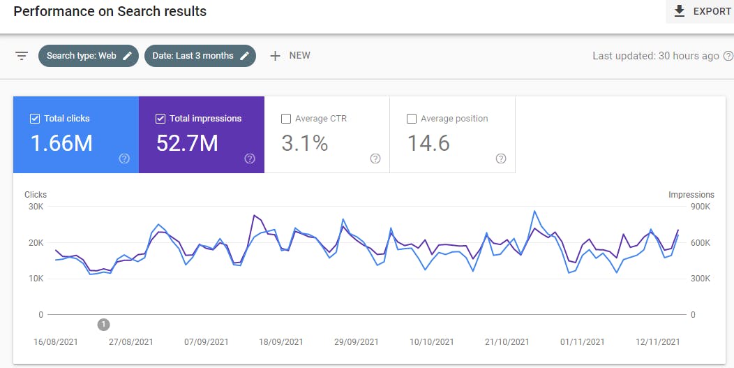 Search console's interface organizes data across metrics such as
- Impressions,
- average search results position,
- CTR,
- and clicks
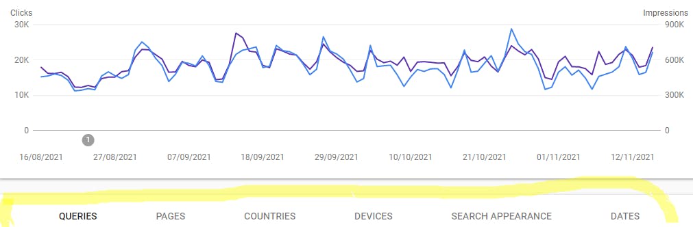
The dimensions across which the metrics are organized include:
- Queries,
- pages,
- countries,
- devices,
- search appearance, and dates.
 Due to some permeability problems in the UI, search console is not the best place for deep performance diagnostics. Search console's UI also poses limitations on the scope and interrelatedness of data that can be exported i.e. You can't download the queries, pages, countries, et cetera, all at once
To bypass this challenge, we'll be using a chrome extension to improve the depth of the data we can export.
- In the google workspace marketplace, search for Search Analytics For Sheets
- Install it on a google account you own
- Open google sheets in the associated google account and under extension>Add ons>click open in sidebar and you’ll get
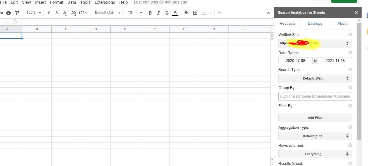 Start by choosing a one-month date range and then choose all the dimensions that are available. Note how these dimensions correspond to everything in GSC.
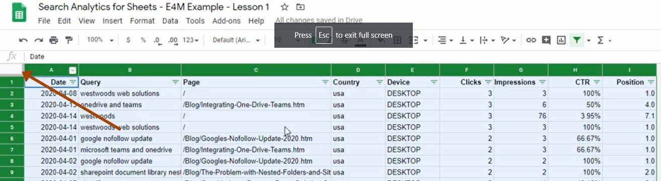
On downloading the data in excel, you’ll get something that looks like this
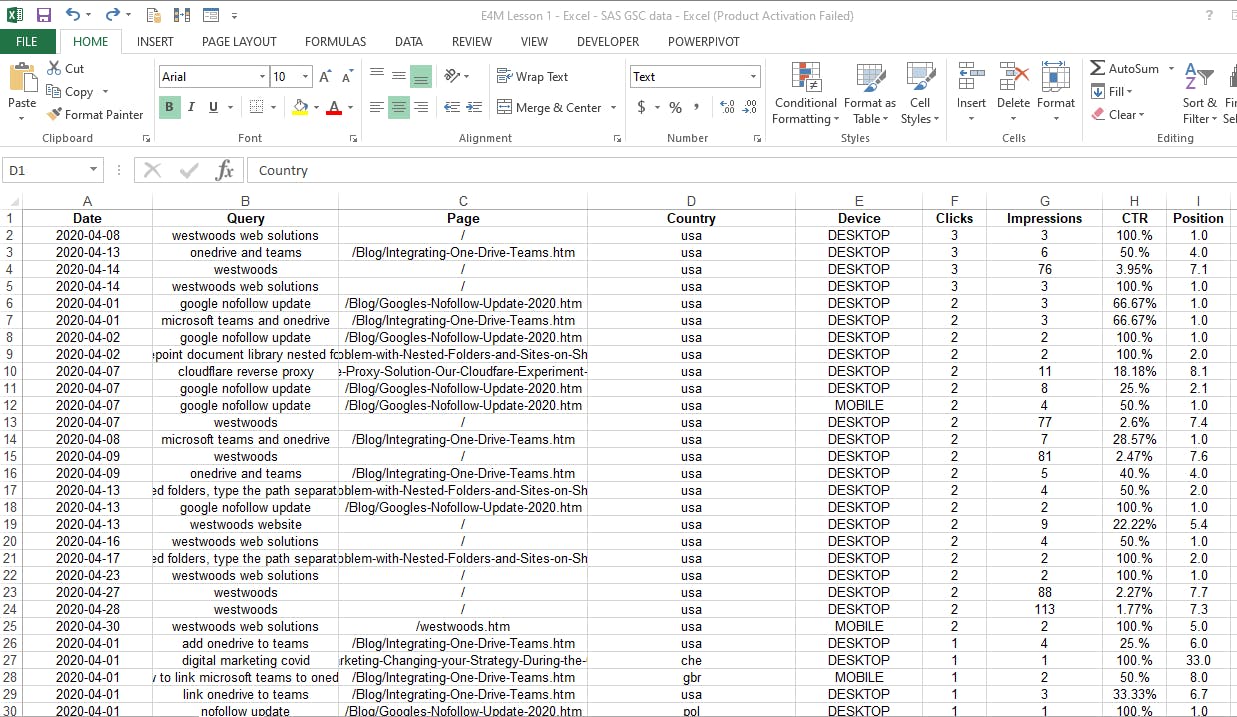 Now that the data is ready, let's explore using some inbuilt operators and functions
**GSC – Sort and Filter
Sorting **
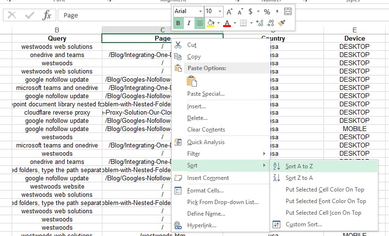
Sorts on a multi-column table can be done on several levels. For a one-dimensional sort of let's say, the pages column, here's how you'll do it.
Move the cursor to a cell in the page column > and do a right-click, you’ll get a sort option. Choose Sort by A to Z. Follow the steps in the image below.
 For a multi-level sort i.e. sorting by more than 1 Column, here's how to do it
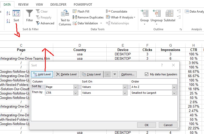 In the image above, I added CTR as the secondary sort level.
**For Filtering
**
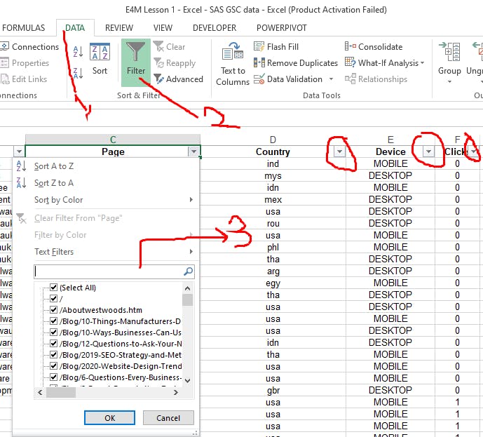
Let's say I wanted to look at just one particular page and want to know what queries pointed to blog posts on Google tag manager. I can use the Filter command to do that. Here’s how
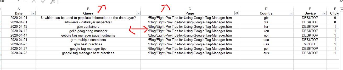
 On filtering for "google tag manager" in the pages column, I get all queries that drive traffic to the page as seen below
 The same operations can be replicated in google sheets but with slight differences
1) Unlike excel, google sheets doesn’t automatically detect that the data is a table so after sorting, the headers would be lost. To let sheets know that it is a table, you'll have to click the button highlighted below
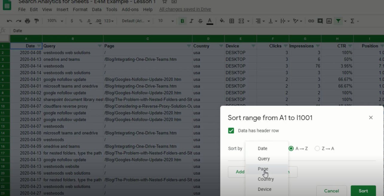
 After highlighting the table, click on the Data command > Sort range > tell it that your table has headers > and then sort by page A to Z.
 Adding filters is similar. We're going to go up to the data command > create a filter, and then we’ll have filters on each column.
SUM & COUNT – Variations Let's explore some variations of the SUM command which are of 3 different types of pl
● SUM (sums everything)
● SUMIF (sums based on one condition)
● SUMIFS (sums based on multiple conditions)
Note:

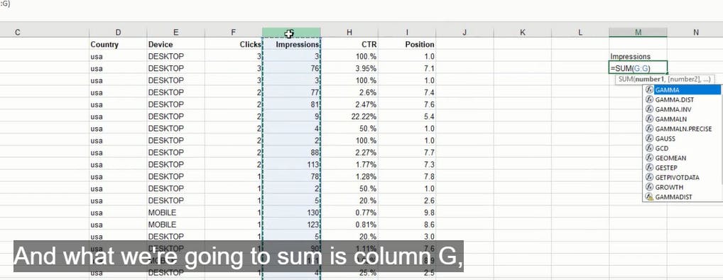
So let's say we want to know how many impressions were served up in the time period that we're looking at. We can do that fairly easily using the Autosum tab in the formulas menu.
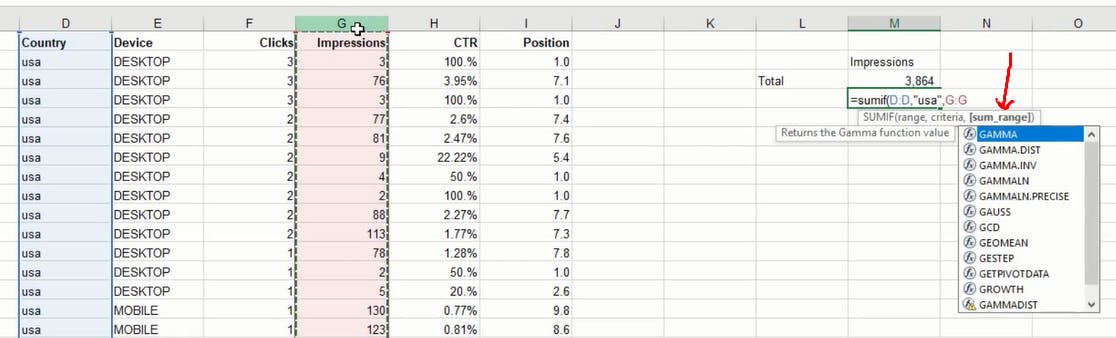
 Let's say, we're curious, how many of those impressions were served up in the U.S.?
That is where we use the SUMIF command, where we get to sum based on one condition, in this case, the country is the USA. We'll start that command by typing the SUMIF command and inputting the required attributes as seen below
 Since we are really smart marketers and data analysts, we know that the key to success is diving further into further segments. So let's break this down by device type, desktop, mobile, and tablet. This is where we would use the SUMIFS command because we're checking on multiple conditions. We're going to check on the country and device type. So we'll use the SUMIFS command.
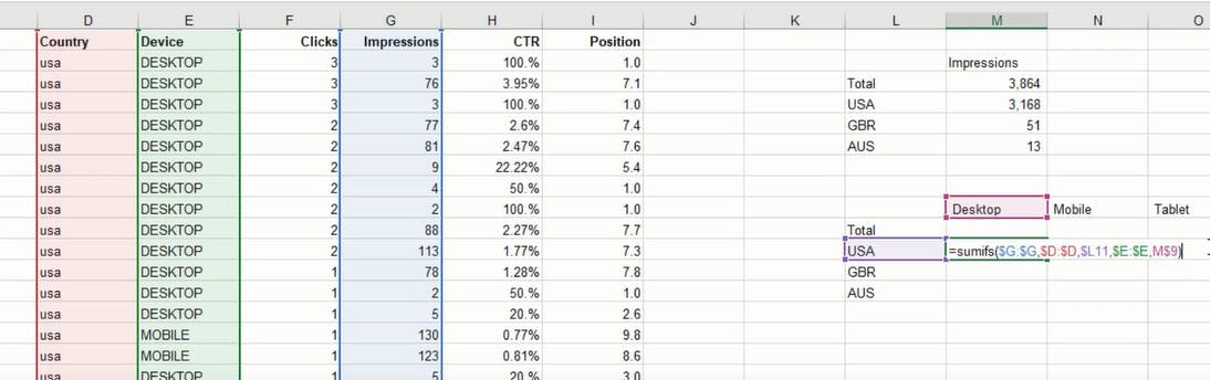 Note: the formula above involved the use of variables as well as relative and absolute cell references.
**De-Dup, Text To Columns, Vlookup & XLookups
**
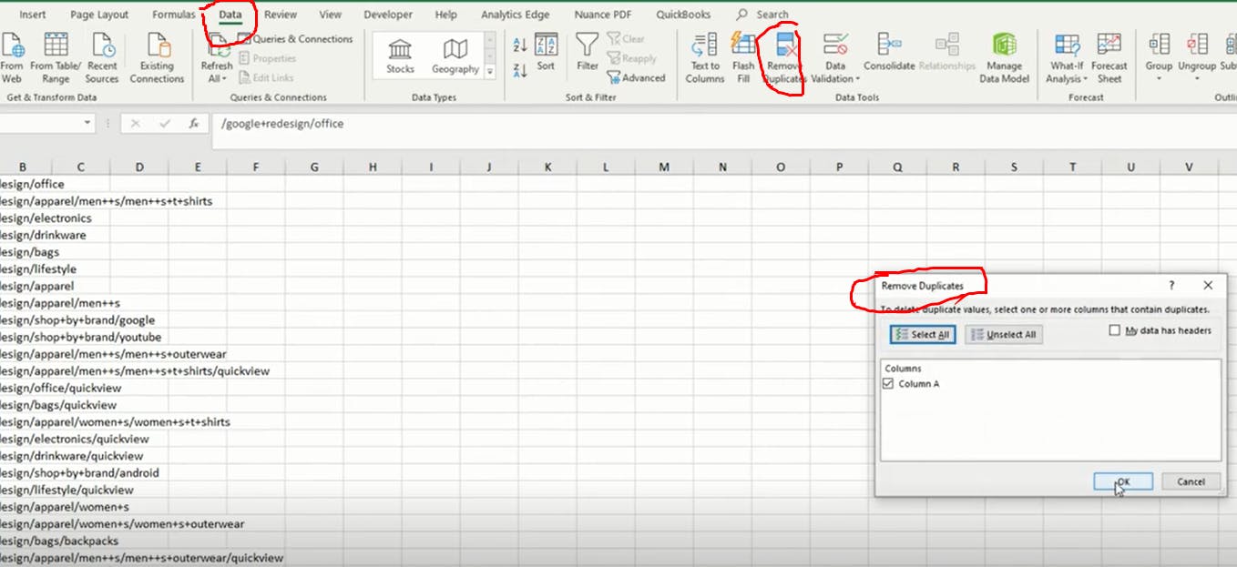
De-duplication is an important operation because of the role it plays in data cleaning. Here's how to go about it
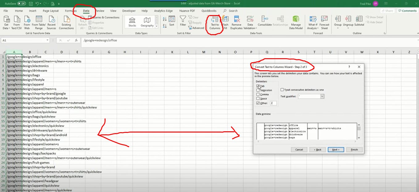
 ### Text To Columns
Converting text to columns is another data cleaning operation that is particularly important when we want to splice chunks of text that do not belong together
Here's out to go about it by using the text-column command under the data tab.
 VLOOKUP
The VLOOKUP function stands for vertical lookup. It allows you to search your table for a certain value and then output its associated value.
If, for example, you are using VLOOKUP with a URL as your lookup value, “Exact Match” is the only way you’ll find the corresponding information for that specific URL — e.g. the page title or the pageviews.
To use VLOOKUP, add a column to your spreadsheet where you will display the found data. Select the first blank cell in this column and click Insert>Function, and then type in VLOOKUP. Once selected, a dialog field will appear allowing you to define four values for your lookup.
**INDEX and MATCH
**
VLOOKUP requires the match to be in the very first column. INDEX and MATCH are specifically used to get around this VLOOKUP limitation.
There are (at least) 3 reasons why Excel experts substitute VLOOKUP with INDEX and MATCH:
1) Unlike VLOOKUP, which searches only to the right, INDEX and MATCH can look in both directions — left and right.
2) INDEX & MATCH can perform two-way lookups by both looking along the rows and along the columns to find the intersection within a matrix.
3) INDEX & MATCH is less prone to errors. Assume you have a VLOOKUP where the final value you want to be returned is in column N. Your lookup value is in column A. You need to highlight the entire A to N range and then provide your index number to be 14. If you happen to delete any of the in-between columns, you would have to update that index number. You don’t need to worry about this when you use INDEX & MATCH.
Note: INDEX and MATCH are more flexible than VLOOKUP.
**XLOOKUP — Excel
**
This function does not exist in Sheets. It was rolled out in August of 2019.
XLOOKUP can search both vertically and horizontally (so, it replaces both VLOOKUP and HLOOKUP). In its simplest form, XLOOKUP needs just 3 arguments to perform the most common exact lookup (one fewer than VLOOKUP). Let’s consider its signature in the simplest form:
XLOOKUP(lookup_value,lookup_array,return_array)
- lookup_value: What you are looking for
- lookup_array: Where to find it
- return_array: What to return
**String Functions
**
String functions are functions that allow you to manipulate blocks of text in different ways. Let’s explain the most valuable of them.
LEN
LEN function is a text function that returns the length of a string/ text.
- =LEN(B3) will calculate the given text or string in cell B3
- =SUM(LEN(B3),LEN(C3),LEN(D3)) will calculate the total number of characters in different cells (B3, C3, and D3 in the given example)
- =LEN(TRIM(B3)) will count characters in excel, excluding leading and trailing spaces
- =LEN(SUBSTITUTE(B3,” “,””)) will count the number of characters in a cell, excluding all spaces
**SUBSTITUTE
**
The SUBSTITUTE function is used to replace a given text with another text in a given cell. It has four parameters:
- text, old_text, new_text are compulsory parameters, and
- instance_num is optional. It specifies the occurrence of old_text. if you specify the instance only, that instance will be replaced by a substitute function; otherwise, all instances are replaced by it.
=SUBSTITUTE(B3,”,” “1) will replace the first instance of “” with space
=SUBSTITUTE(B3,”,” “) will replace all instances of “” with space
Note:
The SUBSTITUTE function is the case-sensitive function!
SUBSTITUTE function does not support wildcard characters (i.e. “?”,“*”)
### FIND
The FIND function in excel is used to find the location of a character or a substring in a text string. It returns the position of the 1st occurrence of find_text in within_text, and has three parameters:
- find_text: The text to find.
- within_text: The text string to be searched within
- start_num: (optional) It specifies from which character the search shall begin. The default is one.
Note:
As the SUBSTITUTE function, the FIND function is also case sensitive and does not allow wildcard characters
If the find_text contains more than one character, the position of the 1st character of the 1st match in within_text is returned.
If find_text is an empty string “”, the FIND function will return one.
If the Excel FIND function cannot find find_text in within_text, it gives #VALUE! error
If the start_num is zero, negative, or greater than within_text, the FIND function returns #VALUE! error.
### SEARCH
The SEARCH function is a text function, which is used to find the location of a substring in a string/text. It has three parameters: find_text and within_text are compulsory parameters and start_num is optional.
- find_text: refers to the substring or character which you want to search within a string or the text you want to find out.
- within_text: where your substring is located or where you perform the find_text.
- start_num: from where you want to start the SEARCH within the text in excel. if omitted, then SEARCH considers it as 1 and starts searching from the first character.
**Error Trapping
** If you lock a whole spreadsheet, users will be able to see the data in the spreadsheet but not be able to enter additional data. You can unlock sections of the spreadsheet to allow data input. Named ranges, which are one of the distinguishing marks of the spreadsheet-power-user, can be used all over the place, not just in pivot tables. VLOOKUP, XLOOKUP, and multiple other applications come to mind. The one thing they can’t have is spaces — or dashes — in their name.
Additional Resources
- Ben Collins — Google Sheets developer blog
- Google sheets help center
- Excel help & learning
- Analytics Edge
- G Suite marketplace
Conclusion
You can’t have good analytical skills and be bad at Excel and/or Sheets. This is why competence in at least one of these applications should be part of every marketer's personal development goals.###